Run GWSWUSE (under development)

Installing GWSWUSE

Installation Steps

Follow these steps to to install ReGWSWUSE:

1) Install Python and download libraries

Download the latest version of Python from the official Python website and install it if Python is not already installed on your system.

2) Clone the ReGWSWUSE repository

Using the Terminal, navigate to the directory of choice where the ReGWSWUSE folder will be copied into. Then use the following command to clone the repository.

$ git clone https://github.com/HydrologyFrankfurt/ReGWSWUSE

Find more information in the official GitHub documentation here .

3) Create an environment to run ReGWSWUSE in

Navigate to the ReGWSWUSE folder in the terminal using the following command.

$ cd user/…/ReGWSWUSE

Create an environment (e.g. with the name “regwswuse”) and install the required packages from the requirements.txt file by running the following command.

example

$ mamba create --name regwswuse --file requirements.txt

Activate the ReGWSWUSE environment using the following command.

example

$ mamba activate regwswuse

Preparing the Input Data

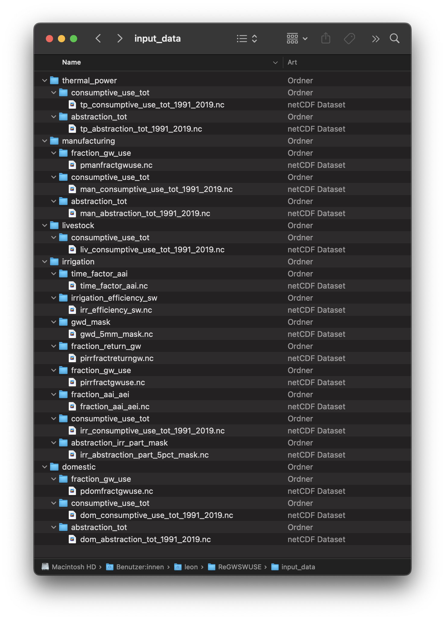
Input data must be located in a specified folder path indicated in the configuration file, following a defined directory structure. The structure of the input folder is precisely defined in the convention file (gwswuse_convention). It is based on a hierarchical organization by sectors and variables:

• Sector Requirements: The sector names in the convention file specify which sector subfolders must be searched in the input data path. For example, the subfolder irrigation corresponds to the irrigation sector, while domestic refers to the household sector.

• Expected Variables: The expected variables specify from which variable subfolders within each sector NetCDF files should be read. These subfolders represent specific data categories, such as consumptive_use_tot (total consumptive water use), fraction_gw_use (fraction of consumptive groundwater use), etc.

When the data is placed in the input_data folder correctly, it will look like this:

Needs to be provided by the User - consumptive_use_tot: [m³/month], monthly data (monthly potential irrigation consumptive water use)

Already provided in the cloned github input data folder <link>. User can provide their own if they want to. - fraction_gw_use: [-], time-invariant (potential irrigation fraction of groundwater use) - fraction_return_gw: [-], time-invariant (potential irrigation fraction of return flow to groundwater) - irrigation_efficiency_sw: [-], time-invariant (Irrigation efficiency for surface water abstraction infrastructure) - gwd_mask: [boolean], time-invariant (mask for groundwater depletion due to human water use greater than 5 mm/yr average for 1980–2009) - abstraction_irr_part_mask: [boolean], time-invariant (mask for irrigation part of water abstraction greater than 5% during 1960–2000)

Needs to be provided by the User - consumptive_use_tot: [m³/year], yearly data (yearly potential domestic consumptive water use) - abstraction_tot: [m³/year], yearly data (yearly potential domestic water abstraction)

Already provided in the cloned github input data folder <link>. User can provide their own if they want to. - fraction_gw_use: [-], time-invariant (potential domestic fraction of groundwater use)

Needs to be provided by the User - consumptive_use_tot: [m³/year], yearly data (yearly potential manufacturing consumptive water use) - abstraction_tot: [m³/year], yearly data (yearly potential manufacturing water abstraction)

Already provided in the cloned github input data folder <link>. User can provide their own if they want to. - fraction_gw_use: [-], time-invariant (potential manufacturing fraction of groundwater use)

Needs to be provided by the User - consumptive_use_tot: [m³/year], yearly data (yearly potential thermal power consumptive water use) - abstraction_tot: [m³/year], yearly data (yearly potential thermal power water abstraction)

Needs to be provided by the User - consumptive_use_tot: [m³/year], yearly data (yearly potential livestock consumptive water use)

Additional Required Input Data for Other Configuration Settings

If other configuration options are set, additional input data will be required, specifically for the irrigation sector:

Irrigation:

• fraction_aai_aei: [-], monthly data (fraction of areas actually irrigated to areas equipped for irrigation for 1901-2020)

• time_factor_aai: [-], monthly data (temporal development factor of national areas actually irrigated for 2016-2020 relative to 2015)

Optional Input Data

For the sectors domestic, manufacturing, livestock, and thermal power, sector-specific fraction_gw_use and fraction_return_gw can also be provided as optional input data. This requires the creation of a variable folder within the respective sector subfolders and placing the corresponding netCDF file in that folder.

Running the Software

The simulation in ReGWSWUSE is executed via the main program run_gwswuse.py. This script manages the entire simulation process and ensures that all modules and functions are called and executed in the correct order. This chapter explains how the main script works and how to use it to run the simulation.

Before you run the simulation, make sure the previously described steps have been completed.

• Installation Completed: Ensure that ReGWSWUSE has been successfully installed per the installation instructions (see Chapter 2.2).

• Configuration File preparation: Prepare the JSON configuration file containing all necessary settings for your simulation. This file should define paths to input data, the simulation period, specific simulation options, and output directories (see the “Configuration Module and File” chapter). Save the configuration file in the same directory as run_gwswuse.py.

• Input Data preparation: Ensure that the folder specified by cm.input_data_path in the configuration file is populated with the required input files. These files must meet the requirements set forth in the convention file (gwswuse_convention), including correct structure, variable names, units, and required spatial and temporal coverage.

WaterGap-2.2e mode

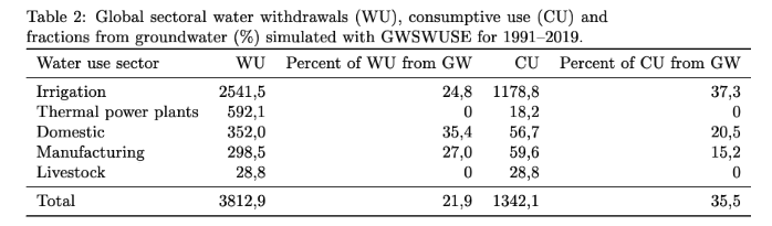
This example reproduces Table 6 from the WatergGAP 2.2.e paper [1], presenting global sectoral water withdrawals (WU), consumptive water use (CU), and groundwater use fractions as simulated by WaterGAP v2.2e for the period 1991–2019.

The required data processing steps are applied to generate aggregated values for water withdrawals and consumptive use over time.

In the 2.2.e paper [1], monthly potential irrigation consumptive water use values are already scaled by the annual relative shares of AAI to AEI (fraction_aai_aei). The dataset used provides corrected values for irrigation consumptive use from 2006 onward.

Prerequisites: You will need to clone ReGWSWUSE and create an environment to run it in. If you haven’t done so already follow the tutorial above for this.

1) Prepare the input data

Download all required input data, remove all leap days, and place the data in the “input_data” folder in your ReGWSWUSE repository as explained above.

2) Set up the configuration file

To configure ReGWSWUSE, go to your ReGWSWUSE repository and navigate to “gwswuse_config.json” and open the configuration file.

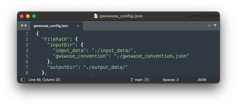
2.1) File Paths

The first options in the configuration file regard input and output file paths. In this example, we will leave them unmodified. The locations for input and output data can be seen in the picture below.

2.2) Simulation Options

Under “SimulationOption” set the parameters to match those in the picture below.

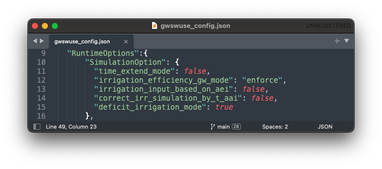
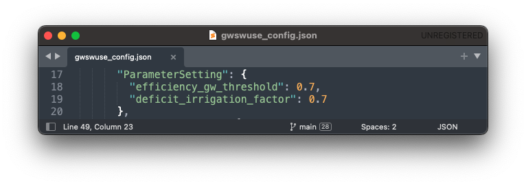
2.3) Parameter Settings

Under “ParameterSetting” set “efficiency_gw_threshold” to “0.7” and “deficit_irrigation_factor” to “0.7”.

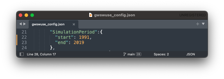
2.4) Simulation Period

In this example we are running the simulation for the years 1991-2019. Under “SimulationPeriod” change the “start” date to “1991” and the “end” date to “2019”.

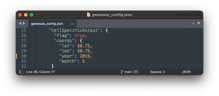
2.5) Cell Specific Output

“CellSpecificOutput” does not need to be changed.

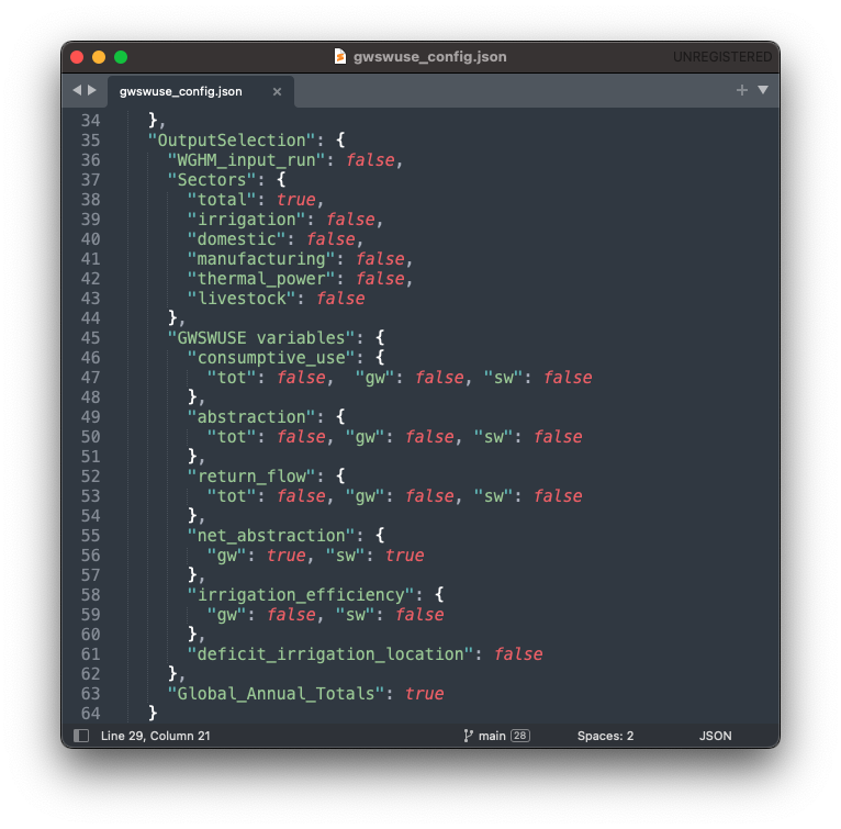
2.6) Output Selection

Under “OutputSelection”, set the parameters as shown in the picture below.

3) Run the simulation

Navigate to your ReGWSWUSE folder in the terminal, activate your environment, and run ReGWSWUSE using the following command:

$ python run_gwswuse.py gwswuse_config.json

Checking Execution

Console Output:

During execution, the software will output progress and important information to the console. Pay attention to any error messages or indications that adjustments may be needed.

Result Storage:

The results will be saved in the output folder defined in the configuration file (cm.output_dir) and can subsequently be analyzed.

By flexibly adjusting the configuration file and using the main script run_gwswuse.py with the specified configuration file, you can adapt the simulation to a variety of scenarios and requirements, making ReGWSWUSE a versatile tool for modeling water use. Some of which are listed below.

4) Results

The goal of this tutorial is to reproduce the results presented in the WaterGAP 2.2e Paper [1], which are shown in the following table:

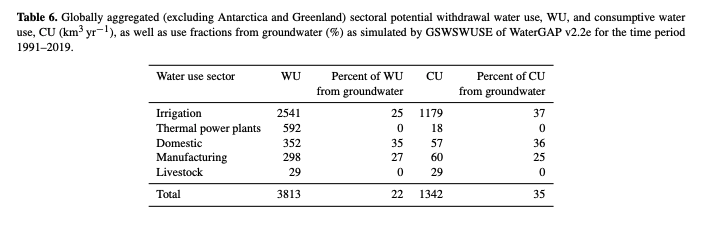
In the output folder, set in Step 2.1, you will find the “global_annual_totals.xlsx” Excel file.

The Consumptive total water use (CU) data can be found in the “consumptive_use_tot” sheet. The total water abstraction (WU) data can be found in the “abstraction_tot” sheet. To reproduce Table 6 we will firstly calculate the mean values for each of the five sectors (irrigation, domestic, manufacturing, thermal power and livestock) by dividing the sum by the number of years (here: 29 from 1991 to 2019). The calculated values correspond closely to the expected results presented in the paper as seen below:

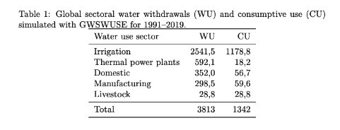
The consumptive total groundwater use and water abstraction from groundwater data can be found in the “consumptive_use_gw” and “abstraction_gw” sheets. The percentages of CU and WU from groundwater use can be calculated by dividing the mean value from groundwater groundwater abstractions for each sector by the total mean values and are shown in the table below. They too closely correspond to the expected results.

Standard Mode (Updated later)

References

[1] (1,2,3)

Müller Schmied, H., Trautmann, T., Ackermann, S., Cáceres, D., Flörke, M., Gerdener, H., Kynast, E., Peiris, T. A., Schiebener, L., Schumacher, M., and Döll, P.: The global water resources and use model WaterGAP v2.2e: description and evaluation of modifications and new features, Geosci. Model Dev., 17, 8817–8852, https://doi.org/10.5194/gmd-17-8817-2024, 2024.